
Figure 5.6-1: Three departmental Ethernets interconnected with a hub.
Figure 5.6-1 shows how three academic departments in a university might interconnect their LANs. In this figure, each of the three departments has a 10BaseT Ethernet that provides network access to the faculty, staff and students of the departments. Each host in a department has a point-to-point connection to the departmental hub. A fourth hub, called a backbone hub, has point-to-point connections to the departmental hubs, interconnecting the LANs of the three departments. The design shown in Figure 5.6-1 is a multi-tier hub design because the hubs are arranged in a hierarchy. It is also possible to create multi-tier designs with more than two tiers -- for example, one tier for the departments, one tier for the schools within the university (e.g., engineering school, business school, etc.) and one tier at the highest university level. Multiple tiers can also be created out of 10Base2 (bus topology Ethernets) with repeaters.
In a multi-tier design, we refer to the entire interconnected network as a LAN, and we refer to each of the departmental portions of the LAN (i.e., the departmental hub and the hosts that connect to the hub) as a LAN segment. It is important to note that all of the LAN segments in Figure 5-6.1 belong to the same collision domain, that is, whenever two or more nodes on the LAN segments transmit at the same time, there will be a collision and all of the transmitting nodes will enter exponential backoff.
Interconnecting departmental LANs with a backbone hub has many benefits. First and foremost, it provides inter-departmental communication to the hosts in the various departments. Second, it extends the maximum distance between any pair of nodes on the LAN. For example, with 10BaseT the maximum distance between a node and its hub is 100 meters; therefore, in a single LAN segment the maximum distance between any pair of nodes is 200 meters. By interconnecting the hubs, this maximum distance can be extended, since the distance between directly-connected hubs can also be 100 meters when using twisted pair (and more when using fiber). Third, the multi-tier design provides a degree of graceful degradation. Specifically, if any one of the departmental hubs starts to malfunction, the backbone hub can detect the problem and disconnect the departmental hub from the LAN; in this manner, the remaining departments can continue to operate and communicate while the faulty departmental hub gets repaired.
Although a backbone hub is a useful interconnection device, it has three serious limitations that hinder its deployment. First, and perhaps more important, when departmental LANs are interconnected with a hub (or a repeater), then the independent collision domains of the departments are transformed into one large and common collision domain. Let us explore this latter issue in the context of Figure 5.6-1. Before interconnecting the three departments, each departmental LAN had a maximum throughput of 10 Mbps, so that maximum aggregate throughput of the three LANs was 30 Mbps. But once the three LANs are interconnected with a hub, all of the hosts in the three departments belong to the same collision domain, and the maximum aggregate throughput is reduced to 10 Mbps.
A second limitation is that if the various departments use different Ethernet technologies, then it may not be possible to interconnect the departmental hubs with a backbone hub. For example, if some departments use 10BaseT and the remaining departments use 100BaseT, then it is impossible to interconnect all the departments without some frame buffering at the interconnection point; since hubs are essentially repeaters and do not buffer frames, they cannot interconnect LAN segments operating at different rates.
A third limitation is that each of the Ethernet technologies (10Base2, 10BaseT, 100BaseT, etc.) has restrictions on the maximum number of nodes that can be in a collision domain, the maximum distance between two hosts in a collision domain, and the maximum number of tiers that can be present in a multi-tier design. These restrictions constrain both the total number of hosts that connect to a multi-tier LAN as well as geographical reach of the multi-tier LAN.
Figure 5.6-2 shows how the three academic departments of our previous
example might be interconnected with a bridge. The three numbers next to
the bridge are the interface numbers for the three bridge interfaces. When
the departments are interconnected by a bridge, as in Figure 5.6-2, we
again refer to the entire interconnected network as a LAN, and we again
refer to each of the departmental portions of the network as LAN segments.
But in contrast to the multi-tier hub design in Figure 5.6-1, each LAN
segment is now an isolated collision domain.

Figure 5.6-2: Three departmental LANs interconnected with a
bridge.
Bridges can overcome many of the problems that plague hubs. First, bridges permit inter-departmental communication while preserving isolated collision domains for each of the departments. Second, bridges can interconnect different LAN technologies, including 10 Mbps and 100 Mbps Ethernets. Third, there is no limit to how big a LAN can be when bridges are used to interconnect LAN segments: in theory, using bridges, it is possible to build a LAN that spans the entire globe.
|
|
|
|
|
|
|
|
|
|
|
|
|
|
|
|
To understand how bridge filtering and forwarding works, suppose a frame with destination address DD-DD-DD-DD-DD-DD arrives to the bridge on interface x. The bridge indexes its table with the LAN address DD-DD-DD-DD-DD-DD and finds the corresponding interface y.
Let's walk through these rules for the network in Figures 5.6-2 and its bridge table in Figure 5.6-3. Suppose that a frame with destination address 62-FE-F7-11-89-A3 arrives to the bridge from interface 1. The bridge examines its table and sees that the destination is on the LAN segment connected to interface 1 (i.e., the Electrical Engineering LAN). This means that the frame has already been broadcast on the LAN segment that contains the destination. The bridge therefore filters (i.e., discards) the frame. Now suppose a frame with the same destination address arrives from interface 2. The bridge again examines its table and sees that the destination is the direction of interface 1; it therefore forwards the frame to the output buffer preceding interface 1. It should be clear from this example that as long as the bridge table is complete and accurate, the bridge isolates the departmental collision domains while permitting the departments to communicate.
Recall that when a hub (or a repeater) forwards a frame onto a link, it just sends the bits onto the link without bothering to sense whether another transmission is currently taking place on the link. In contrast, when a bridge wants to forward a frame onto a link, it runs the CSMA/CD algorithm discussed in Section 5.3. In particular, the bridge refrains from transmitting if it senses that some other node on the LAN segment is transmitting; furthermore, the bridge uses exponential backoff when one of its transmissions results in a collision. Thus bridge interfaces behave very much like node adapters. But technically speaking, they are not node adapters because neither a bridge nor its interfaces have LAN addresses. Recall that a node adapter always inserts its LAN address into the source address of every frame it transmits. This statement is true for router adapters as well as host adapters. A bridge, on the other hand, does not change the source address of the frame.
One significant feature of bridges is that they can be used to combine Ethernet segments using different Ethernet technologies. For example, if in Figure 5.6-2, Electrical Engineering has a 10Base2 Ethernet, Computer Science has a 100BaseT Ethernet, and Electrical Engineering has a 10BaseT Ethernet, then a bridge can be purchased that can interconnect the three LANs. With Gigabit Ethernet bridges, it is possible to have an additional 1 Gbps connection to a router, which in turn connects to a larger university network. As we mentioned earlier, this feature of being able to interconnect different link rates is not available with hubs.
Also, when bridges are used as interconnection devices, there is no theoretical limit to the geographical reach of a LAN. In theory, we can build a LAN that spans the globe by interconnecting hubs in a long, linear topology, with each pair of neighboring hubs interconnected by a bridge. Because in this design each of the hubs has its own collision domain, there is no limit on how long the LAN can be. We shall see shortly, however, that it is undesirable to build very large networks exclusively using bridges as interconnection devices -- large networks need routers as well.
|
|
|
|
|
|
|
|
|
|
|
|
|
|
|
|
|
|
|
|
Continuing with this same example, suppose that the aging time for this bridge is 60 minutes and no frames with source address 62-FE-F7-11-89-A3 arrive to the bridge between 9:32 and 10:32. Then at time 10:32 the bridge removes this address from its table.
Bridges are plug and play devices because they require absolutely no intervention from a network administrator or user. When a network administrator wants to install a bridge, it does no more than connect the LAN segments to the bridge interfaces. The administrator does not have to configure the bridge tables at the time of installation or when a host is removed from one of the LAN segments. Because bridges are plug and play, they are also referred as transparent bridges.

Figure 5.6-5: Interconnected LAN segments with redundant paths.
Multiple redundant paths between LAN segments (such as departmental LANs) can greatly improve fault tolerance. But, unfortunately, multiple paths have a serious side effect -- frames cycle and multiply within the interconnected LAN, thereby crashing the entire network [Permian 1999]. To see this, suppose that the bridge tables in Figure 5.6-5 are empty, and a host in Electrical Engineering sends a frame to a host in Computer Science. When the frame arrives to the Electrical Engineering hub, the hub will generate two copies of the frame and send one copy to each of the two bridges. When a bridge receives the frame, it will generate two copies, send one copy to the Computer Science hub and the other copy to the Systems Engineering hub. Since both bridges do this, there will be four identical frames in the LAN. This multiplying of copies will continue indefinitely since the bridges do not know where the destination host resides. (To route the frame to the destination host in Computer Science, the destination host has to first generate a frame so that its address can be recorded in the bridge tables.) The number of copies of the original frame grows exponentially fast, crashing the entire network.
To prevent the cycling and multiplying of frames, bridges use a spanning
tree protocol [Permian 1999]. In the spanning
tree protocol, bridges communicate with each other over the LANs in
order to determine a spanning tree, that is, a subset of the original topology
that has no loops. Once the bridges determine a spanning tree, the bridges
disconnect appropriate interfaces in order to create the spanning tree
out of the original topology. For example, in Figure 5.6-5, a spanning
tree is created by having the top bridge disconnect its interface
to Electrical Engineering and the bottom bridge disconnect its interface
to Systems Engineering. With the interfaces disconnected and the loops
removed, frames will no longer cycle and multiply. If, at some later time,
one of links in the spanning tree fails, the bridges can reconnect the
interfaces, run the spanning tree algorithm again, and determine a new
set of interfaces that should be disconnected.
Even though bridges and routers are fundamentally different, network administrators must often choose between them when installing an interconnection device. For example, for the network in Figure 5.6-2, the network administrator could have just as easily used a router instead of a bridge. Indeed, a router would have also kept the three collision domains separate while permitting interdepartmental communication. Given that both bridges and routers are candidates for interconnection devices, what are the pros and cons of the two approaches?
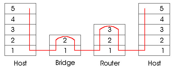
First consider the pros and cons of bridges. As mentioned above, bridges are plug and play, a property that is cherished by all the over-worked network administrators of the world. Bridges can also have relatively high packet filtering and forwarding rates -- as shown in Figure 5.6-6, bridges only have to process packets up through layer 2, whereas routers have to process frames up through layer 3. On the other hand, the spanning tree protocol restricts the effective topology of a bridged network to a spanning tree. This means that all frames most flow along the spanning tree, even when there are more direct (but disconnected) paths between source and destination. The spanning tree restriction also concentrates the traffic on the spanning tree links when it could have otherwise been spread through all the links of the original topology. Furthermore, bridges do not offer any protection against broadcast storms -- if one host goes haywire and transmits an endless stream of Ethernet broadcast packets, the bridges will forward all of the packets and the entire network will collapse.
Now consider the pros and cons of routers. Because IP addressing is hierarchical (and not flat as is LAN addressing), packets do not normally cycle through routers even when the network has redundant paths. (Actually, packets can cycle when router tables are misconfigured; but as we learned in Chapter 4, IP uses a special datagram header field to limit the cycling.) Thus, packets are not restricted to a spanning tree and can use the best path between source and destination. Because routers do not have the spanning tree restriction, routers have allowed the Internet to be built with a rich topology which includes, for example, multiple active links between Europe and North America. Another feature of routers is that they provide firewall protection against layer-2 broadcast storms. Perhaps the most significant drawback of routers is that they are not plug and play -- they and the hosts that connect to them need their IP addresses to be configured. Also, routers often have a larger prepackage processing time than bridges, because they have to process up through the layer-3 fields. Finally, there are two different ways to pronounce the word "router", either as "rootor" or as "rowter", and people waste a lot of time arguing over the proper pronunciation [Perlman 1999].
Given that both bridges and routers have their pros and cons, when should
an institutional network (e.g., university campus network or a corporate
campus network) use bridges, and when should it use bridges? Typically,
small networks consisting of a few hundred hosts have a few LAN segments.
Bridges suffice for these small networks, as they localize traffic and
increase aggregate throughput without requiring any configuration of IP
addresses. But larger networks consisting of thousands of hosts typically
include routers within the network (in addition to bridges). The routers
provide a more robust isolation of traffic, control broadcast storms, and
use more "intelligent" routes among the hosts in the network.
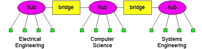
Figure 5.6-7: An example of an institutional LAN without
a backbone.
One important principle when designing an interconnected LAN is that the various LAN segments should be interconnected with a backbone. A backbone is a network that has direct connections to all the LAN segments. When a LAN has a backbone, then each pair of LAN segments can communicate without passing through a third-party LAN segment. The design shown if Figure 5.6-2 uses a three-interface bridge for a backbone. In the homework problems at the end of this chapter we shall explore how to design backbone networks with two-interface bridges.
Switches can be purchased with various combinations of 10 Mbps, 100 Mbps and 1 Gbps interfaces. For example, you can purchase switches with four 100 Mbps interfaces and twenty 10 Mbps interfaces; or switches with four 100 Mbps interfaces and one 1 Gbps interface. Of course, the more the interfaces and the higher transmission rates of the various interfaces, the more you pay. Many switches also operate in a full-duplex mode; that is, they can send and receive frames at the same time over the same interface. With a full duplex switch (and corresponding full duplex Ethernet adapters in the hosts), host A can send a file to host B while that host B simultaneously sends to host A.
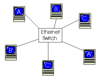
One of the advantages of having a switch with a large number of interfaces is that it creates direct connections between hosts and the switch. When a host has a full-duplex direct connection to a switch, it can transmit (and receive) frames at the full transmission rate of its adapter; in particular, the host adapter always senses an idle channel and never experiences a collision. When a host has a direct connection to a switch (rather than a shared LAN connection), the host is said to have dedicated access. In Figure 5.6-8, an Ethernet switch provides dedicated access to six hosts. This dedicated access allows A to send a file to A' while that B is sending a file to B' and C is sending a file to C'. If each host has a 10Mbps adapter card, then the aggregate throughput during the three simultaneous file transfers is 30 Mbps. If A and A' have 100 Mbps adapters and the remaining hosts have 10 Mbps adapters, then the aggregate throughput during the three simultaneous file transfers is 120 Mbps.
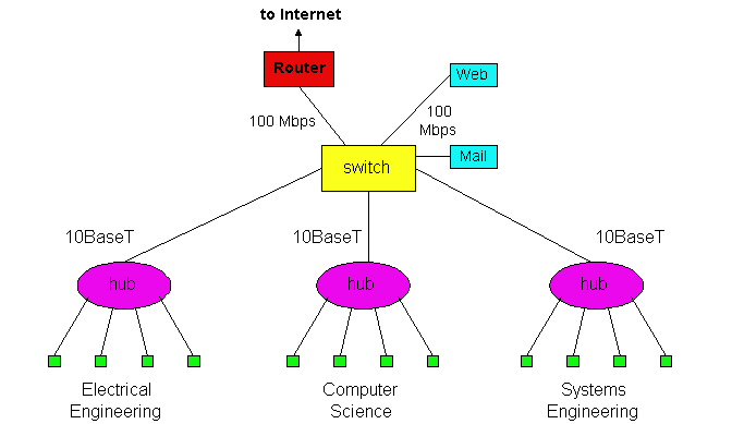
Figure 5.6-9: An institutional network using a combination of
hubs, Ethernet switches and a router.
Figure 5.6-9 shows how an institution with several departments and several
critical servers might deploy a combination of hubs, Ethernet switches
and routers. In Figure 5.6-9, each of the three departments has its own
10 Mbps Ethernet segment with its own hub. Because each departmental hub
has a connection to the switch, all intra-departmental traffic is confined
to the Ethernet segment of the department (assuming the routing tables
in the Ethernet switch are complete). The Web and mail servers each have
dedicated 100 Mbps access to the switch. Finally, a router, leading to
the Internet, has dedicated 100 Mbps access to the switch. Note that this
switch has at least three 10 Mbps interfaces and three100 Mbps interfaces.
Recall from Chapter 1, when a packet is forwarded through a store-and-forward packet switch, the packet is first gathered and stored in its entirety before the switch begins to transmit it on the outbound link. In the case when the output buffer becomes empty before the whole packet has arrived to the switch, this gathering generates a store-and-forward delay at the switch, a delay which contributes to the total end-to-end delay (see Chapter 1). An upper bound on this delay is L/R, where L is the length of the packet and R is transmission rate of the inbound link. Note that a packet only incurs a store-and-forward delay if the output buffer becomes empty before the entire packet arrives to the switch.
With cut-through switching, if the buffer becomes empty before the entire packet has arrived, the switch can start to transmit the front of the packet while the back of the packet continues to arrive. Of course, before transmitting the packet on the outbound link, the portion of the packet that contains the destination address must first arrive. (This small delay is inevitable for all types of switching, as the switch must determine the appropriate outbound link.) In summary, with cut-through switching a packet does not have to be fully "stored" before it is forwarded; instead the packet is forwarded through the switch when the output link is free. If the output link is shared with other hosts (e.g., the output link connects to a hub), then the switch must also sense the link as idle before it can "cut-through" a packet.
To shed some insight on the difference between store-and-forward and cut-through switching, let us recall the caravan analogy introduced in Section 1.6. In this analogy, there is a highway with occasional toll booths, with each toll booth having a single attendant. On the highway there is a caravan of 10 cars traveling together, each at the same constant speed. The cars in the caravan are the only cars on the highway. Each toll booth services the cars at a constant rate, so that when the cars leave the toll booth they are equally spaced apart. As before, we can think of the caravan as being a packet, each car in the caravan as being a bit, and the toll booth service rate as the transmission rate of a link. Consider now what the cars in the caravan do when they arrive to a toll booth. If each car proceeds directly to the toll booth upon arrival, then the toll booth is a "cut-through toll booth". If, on the other hand, each car waits at the entrance until all the remaining cars in the caravan arrive, then the toll booth is "store-and-forward toll booth". The store-and-forward toll booth clearly delays the caravan more than the cut-through toll booth.
A cut-through switch can reduce a packet's end-to-end delay, but
by how much? As we mentioned above, the maximum store-and-forward delay
is L/R, where L is the packet size and R is the rate
of the inbound link. The maximum delay is approximately 1.2 msec for 10
Mbps Ethernet and .12 msec for 100 Mbps Ethernet (corresponding to a maximum
size Ethernet packet). Thus, a cut-through switch only reduces the delay
by .12 to .2 msec, and this reduction only occurs when the outbound link
is lightly loaded. How significant is this delay? Probably not very much
in most practical applications, so you may want to think second about selling
the family house before investing in the cut-through feature.
|
|
|
|
|
|
|
|
|
|
|
|
|
|
|
|
|
|
|
|
|
|
|
|
|
|
|
|
|
|
We have learned in this section that hubs, bridges, routers and switches can all be used as an interconnection device for hosts and LAN segments. Figure 5.6-10 provides a summary of the features of each of these interconnection devices.The Cisco Web site provides numerous comparisons of the different interconnection technologies [Cisco 1999].
Copyright James F. Kurose and Keith W. Ross 1996-1999